Multivariate example
If you want to run the following example on your local machine, you are welcome to download the code here and run it (after having pip-installed pecuzal-embedding and matplotlib packages).
Similar to the approach in the Univariate example, we now highlight the capability of the proposed embedding method for a multivariate input. Again, we define and integrate the ODE’s and restrict ourselves to the first 2,500 samples, in order to save computation time.
import numpy as np
from scipy.integrate import odeint

# integrate Roessler system on standard parameters
def roessler(x,t):
    return [-x[1]-x[2], x[0]+.2*x[1], .2+x[2]*(x[0]-5.7)]

x0 = [1., .5, .5] # define initial conditions
tspan = np.arange(0., 5000.*.2, .2) # time span
data = odeint(roessler, x0, tspan, hmax = 0.01)

data = data[2500:,:]    # remove transients
The idea is now to feed in all three time series to the algorithm, even though this is a very far-from-reality example. We already have an adequate representation of the system we want to reconstruct, namely the three time series from the numerical integration. But let us see what PECUZAL suggests for a reconstruction.
Since we have to deal with three time series now, let us estimate the Theiler window as the maximum of all Theiler windows of each time series. Again, we estimate such a Theiler window by taking the first minimum of the auto mutual information.
import matplotlib.pyplot as plt
from pecuzal_embedding import pecuzal_embedding, mi

N = len(data)
mis = np.empty(shape=(50,3))
for i in range(3):
   mis[:,i], lags = mi(data[:,i])    # compute mutual information up to default maximum time lag

plt.figure(figsize=(14., 8,))

ts_str = ['x','y','z']

cnt = 0
for i in range(0,6,2):
   plt.subplot(3,2,i+1)
   plt.plot(range(1000),data[:1000,cnt])
   plt.grid()
   if i == 4:
      plt.xlabel('time [in sampling units]')
   plt.title(ts_str[cnt]+'-component of Roessler test time series')

   plt.subplot(3,2,i+2)
   plt.plot(lags,mis[:,cnt])
   plt.grid()
   plt.ylabel('MI')
   if i == 4:
      plt.xlabel('time lag [in sampling units]')
   plt.title('Mutual information for '+ts_str[cnt]+'-component of Roessler test time series')
   cnt +=1
plt.subplots_adjust(hspace=.3)
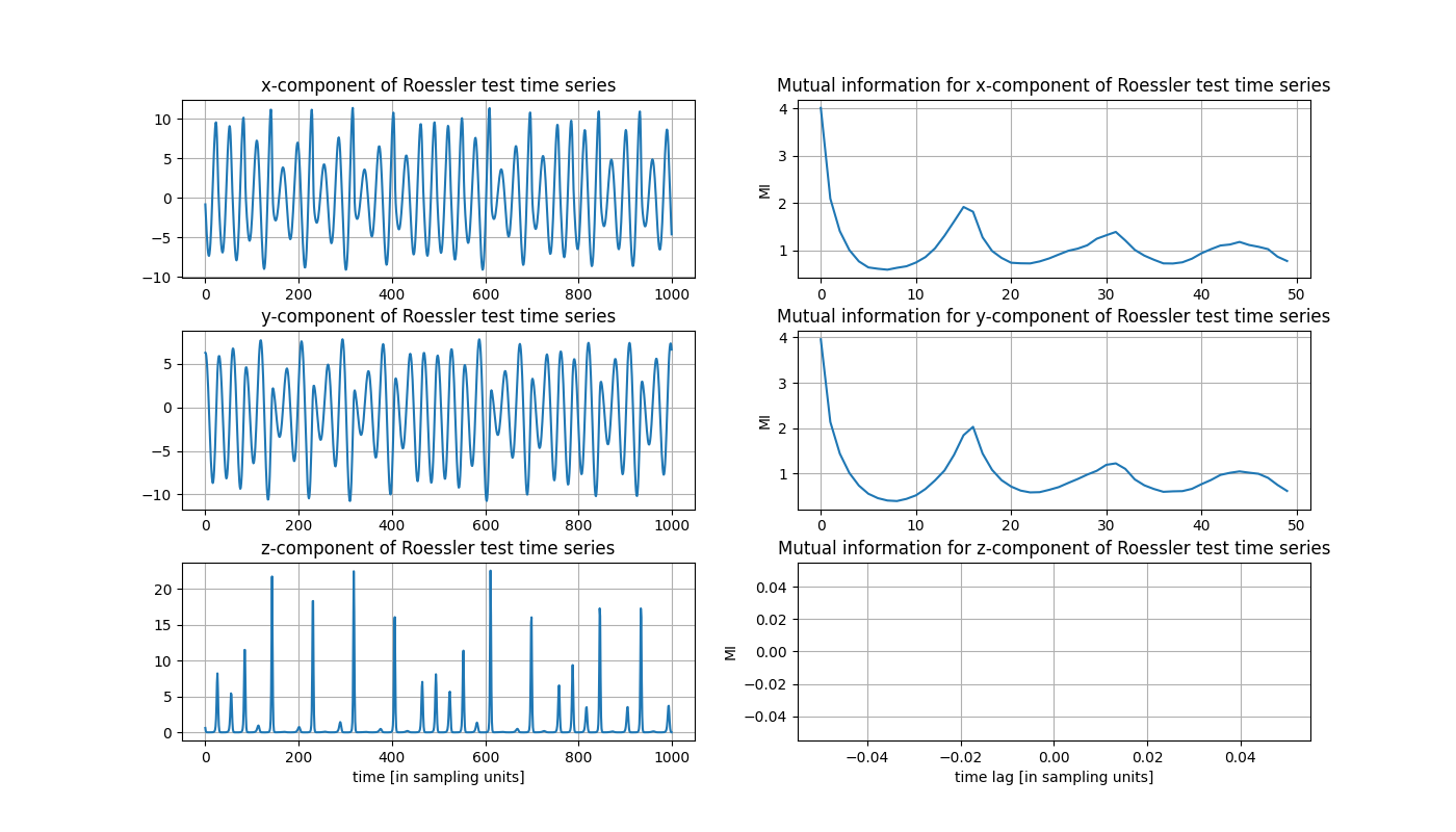
Due to the spikyness of the z-component the according auto mutual information yields nan-values as
a result of empty bins in the histograms. So we stick to the choice of theiler = 7 here and
call the PECUZAL algorithm pecuzal_embedding.pecuzal_embedding() with default kwargs
and possible delays ranging from 0:100. We will run the function with the econ option for faster computation.
NOTE: The following computation will take approximately 70 minutes (depending on the machine you are running the code on).
See also the :ref:`note_performance`.
Y_reconstruct, tau_vals, ts_vals, Ls, eps = pecuzal_embedding(data, taus = range(100), theiler = 7, econ = True)
which leads to the following note in the console:
Algorithm stopped due to increasing L-values. VALID embedding achieved.
The suggested embedding parameters…
tau_vals = [0, 0, 3]
ts_vals = [1, 0, 0]
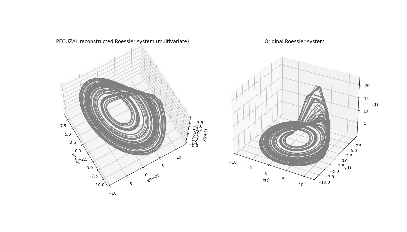
… reveal that PECUZAL builds the reconstructed trajectory Y_reconstruct from the unlagged time series, having index 0, i.e. the y-component and the x-component without lag, and finally again the x-component lagged by 3 samples. As expected the total \(\Delta L\)-value is smaller here than in the univariate case:
L_total_multi = np.sum(Ls)

-1.61236358817
The reconstructed attractor looks also quite similar to the original one, even though that is not a proper evaluation criterion for the goodness of a reconstruction, see [kraemer2021].
from mpl_toolkits import mplot3d

ts_labels = ['x','y','z']

fig = plt.figure(figsize=(14., 8.))
ax = plt.subplot(121, projection='3d')
ax.plot(Y_reconstruct[:,0], Y_reconstruct[:,1], Y_reconstruct[:,2], 'gray')
ax.grid()
ax.set_xlabel('{}(t+{})'.format(ts_labels[ts_vals[0]],tau_vals[0]))
ax.set_ylabel('{}(t+{})'.format(ts_labels[ts_vals[1]],tau_vals[1]))
ax.set_zlabel('{}(t+{})'.format(ts_labels[ts_vals[2]],tau_vals[2]))
ax.set_title('PECUZAL reconstructed Roessler system (multivariate)')
ax.view_init(-115, 30)

ax = plt.subplot(122, projection='3d')
ax.plot(data[:5000,0], data[:5000,1], data[:5000,2], 'gray')
ax.grid()
ax.set_xlabel('x(t)')
ax.set_ylabel('y(t)')
ax.set_zlabel('z(t)')
ax.set_title('Original Roessler system')