Univariate example
If you want to run the following example on your local machine, you are welcome to download the code here and run it (after having pip-installed pecuzal-embedding and matplotlib packages).
We exemplify the proposed embedding method by embedding the y-component of the Roessler system (with standard parameters \([a = 0.2, b = 0.2, c = 5.7]\)). Therefore we define and integrate the ODE’s:
import numpy as np
from scipy.integrate import odeint

# integrate Roessler system on standard parameters
def roessler(x,t):
return [-x[1]-x[2], x[0]+.2*x[1], .2+x[2]*(x[0]-5.7)]

x0 = [1., .5, 0.5] # define initial conditions
tspan = np.arange(0., 5000.*.2, .2) # time span
data = odeint(roessler, x0, tspan, hmax = 0.01)

data = data[2500:,:]    # remove transients
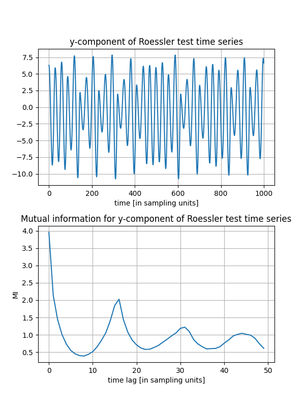
Now bind the time series we would like to consider and compute the auto mutual information, in order to estimate an appropriate Theiler window. This is especially important when dealing with highly sampled datasets. Let’s focus on the first 2,500 samples here and plot the time series and its mutual information:
import matplotlib.pyplot as plt
from pecuzal_embedding import pecuzal_embedding, mi

y = data[:,1]   # bind only y-component
muinf, lags = mi(y)    # compute mutual information up to default maximum time lag

plt.figure(figsize=(6., 8,))
plt.subplot(2,1,1)
plt.plot(range(len(y[:1000])),y[:1000])
plt.grid()
plt.xlabel('time [in sampling units]')
plt.title('y-component of Roessler test time series')

plt.subplot(2,1,2)
plt.plot(lags,muinf)
plt.grid()
plt.ylabel('MI')
plt.xlabel('time lag [in sampling units]')
plt.title('Mutual information for y-component of Roessler test time series')

plt.subplots_adjust(hspace=.3)
Now we are ready to go and simply call the PECUZAL algorithm pecuzal_embedding.pecuzal_embedding()
with a Theiler window determined from the first minimum of the mutual information shown in the above Figure
and possible delays ranging from 0:100. We will run the function with the econ option for faster computation.
NOTE: The following computation will take approximately 13 minutes (depending on the machine you are running the code on).
See also the :ref:`note_performance`.
Y_reconstruct, tau_vals, ts_vals, Ls, eps = pecuzal_embedding(y, taus = range(100), theiler = 7, econ = True)
which leads to the following note in the console:
Algorithm stopped due to increasing L-values. VALID embedding achieved.
Y_reconstruct stores the reconstructed trajectory. Since in this example Y_reconstruct is a three-dimensional trajectory we can actually plot it, in order to visualize the result.
from mpl_toolkits import mplot3d

fig = plt.figure(figsize=(14., 8.))
ax = plt.subplot(121, projection='3d')
ax.plot(Y_reconstruct[:,0], Y_reconstruct[:,1], Y_reconstruct[:,2], 'gray')
ax.grid()
ax.set_xlabel('y(t+{})'.format(tau_vals[0]))
ax.set_ylabel('y(t+{})'.format(tau_vals[1]))
ax.set_zlabel('y(t+{})'.format(tau_vals[2]))
ax.set_title('PECUZAL reconstructed Roessler system')

ax = plt.subplot(122, projection='3d')
ax.plot(data[:5000,0], data[:5000,1], data[:5000,2], 'gray')
ax.grid()
ax.set_xlabel('x(t)')
ax.set_ylabel('y(t)')
ax.set_zlabel('z(t)')
ax.set_title('Original Roessler system')
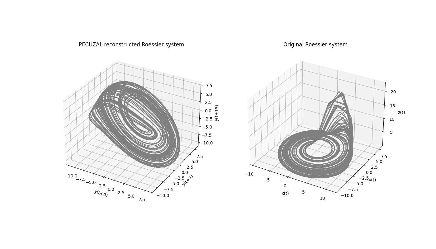
For the correct axis labels we used the delay values the PECUZAL algorithm used and which are stored in the output-variable we named tau_vals above.
tau_vals = [0, 7, 15]
This means, that the reconstructed trajectory consists of the unlagged time series (here the y-component) and two more components with the time series lagged by 7 and 15 samples, respectively. Note the coincidence with the first minimum of the mutual information… The output variable ts_vals stores the chosen time series for each delay value stored in tau_vals. Since there is only one time series we fed in,
ts_vals = [0, 0, 0]
This output is only needed for the multivariate case, see Multivariate example . We can also look at the output of the low-level function, namely the continuity-statistic, which led to the result. We stored these statistics for each embedding cycle in the variable eps.
plt.figure(figsize=(8., 5.))
plt.plot(eps[:,0], label='1st embedding cycle')
plt.scatter([tau_vals[1]], [eps[tau_vals[1],0]])
plt.plot(eps[:,1], label='2nd embedding cycle')
plt.scatter([tau_vals[2]], [eps[tau_vals[2],1]])
plt.plot(eps[:,2], label='3rd embedding cycle')
plt.title('Continuity statistics for PECUZAL embedding of Roessler y-component')
plt.xlabel('delay')
plt.ylabel(r'$\langle \varepsilon^\star \rangle$')
plt.legend(loc='upper right')
plt.grid()
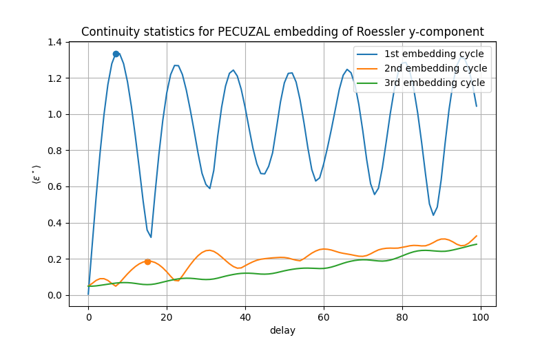
The points mark the postitions, where the algorithm picked the delays for the reconstruction from. In the third embedding cycle there is no delay value picked and the algorithm breaks, because it can not minimize the L-statistic further. Its values for each embedding cycle are stored in Ls:
Ls = [-0.89078493296554, -0.6889087842665718]
Note that the very last value of the \(\Delta L\) values corresponds to the last encountered embedding cycle, that led to a negative \(\Delta L\), i.e. in this case two embedding cycles had been run successful, resulting in a three-dimensional embedding. The total deacrease in L is simply
L_total_uni = np.sum(Ls)

-1.57968927756